Nobody likes sitting on the train, or in traffic, for hours on end each morning and evening.  Beyond being a pain, long commutes can have fairly severe deleterious effects, and are linked to raised rates of obesity, stress, and depression.  It’s not too much of a stretch, then, to imagine that people will pay more to be closer to work, but how much more? This week, we will test out this idea quantitatively, using Chicago as a template.

Chicago makes a nice case study to probe the effects of transit time on housing prices.  The city has a fairly strong public transportation system, which is utilized by people with diverse socio-economic backgrounds.  Also, a large amount of the highest paying jobs are centrally concentrated in or near ‘the Loop’, the medial massif at the heart of the city.  That said, Chicago is a large and extremely diverse city, so it is difficult to completely reproduce housing trends with a fairly simple model (as we are about to do).

To start, we need to get some house price data.  In the age of the internet, home prices and details are abundantly available from online realty services such as Redfin.com and Trulia.com.  Housing prices en masse, however, are actually a coveted resource: detailed, exclusive knowledge of housing availability is a competitive advantage for many realtors, and is guarded somewhat zealously.  This makes retrieving large amounts of house price data for any area a bit of a battle.

Data and Modeling

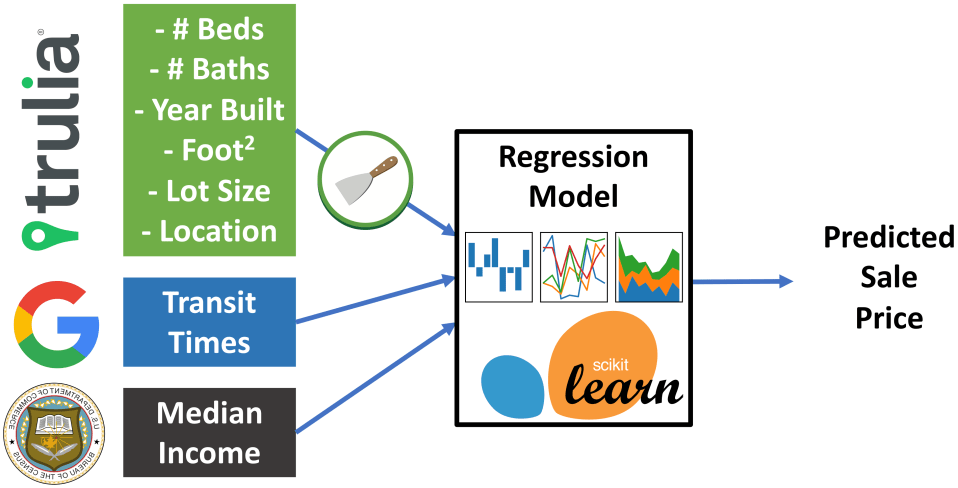
Workflow for regression modeling.

After some consideration, it looks like Trulia.com might be a good accessible source of housing price data, which we can retrieve using the Scrapy web scraping library for python.  With effort, we should be able to retrieve details for ~8000 for sale houses in Chicago. Once this information is in hand for a broad spectrum of houses in Chicago, we need to retrieve travel times using Google’s Directions API.  For this step, we can restrict our hypothetical commuters to public transit, and gave them a moderate affinity for trains over buses. Finally, we can add in zipcode level median incomes, retrieved from the U.S. Census Bureau, as an extra data feature for our modeling efforts.

Once all the data is lined up, downloaded, parsed, and cleaned, we can begin modeling it using the python packages Pandas and Sci-kit Learn.  After building, cross validating a simple linear model, a little feature engineering, and variable elimination using Lasso techniques, we can finally settling on a housing prediction model that only relies on 7 features:

• # Bedrooms
• # Bathrooms
• Square Footage
• Lot Size
• Median Income
• Year Built
• Public Transit Commute Time

Housing price model for all for sale homes in Chicago

Our initial model, although simple, does a decent job of reproducing the general trends expected in the data, with an R² of ~0.6.  That said, there is a ton of scatter in the model.  This really should be expected.  For this model, I’m using a pretty simple set of features, all of which are continuous. This means we are missing a lot.  For example, stone houses with slate roofs are worth a LOT more than wooden houses with corrugated aluminum siding, but our model cannot capture that with the data we have.  Unfortunately, there is not a Chicago equivalent to the superb Ames Housing Dataset, so we must make do with what we have, and limit ourselves to analyzing big picture trends as opposed to making specific predictions.

To try and reduce a little of the scatter in the data, we can restrict ourselves geographically to the north and northwest portions of the city, which are much more socioeconomically homogenous than the city as a whole. This region of the city is largely served by the Chicago Transit Authority’s Red, Brown, and Blue train lines.

Region of further analysis in grey.

The geographic restriction actually reduces the amount of dispersion in our data, raising the R² of our model to ~0.8.

Model of housing prices on Chicago’s north and northwest sides

One clear trend that is consistent with most previous models of housing prices as well as across both of our models: square footage matters a lot.  This seems pretty common sense: bigger houses cost more.

Dependence of model predicted house price on house area

Finally, we get to the crux, the dependence of housing price on transit time:

Dependence of predicted housing price on commute time

Two important takeaways here: in our model, transit times matter a LOT.  First, after square footage, which seems to be the strongest single control on housing price, commute times are the second most important variable, with longer commute times leading to significantly lower house prices on average.  However, there is a lot of dispersion, especially near the city center where transit times are short, but the quality of housing varies greatly.  Second, the most expensive properties in the cities almost exclusively have short, or at least shorter than average, commute times.  This suggests that transit time may play a more important role in determining housing prices at the high end rather than at the low end.  In other words, it is a perk that many are willing to pay for, but only if they have the money.

This is the first in an ongoing series of posts trying to understand the relationship between public transportation and housing prices in the city of Chicago and beyond.